Scikit-learn Tutorial 2026

Installation and Setup of Scikit-learn

You need to set up a virtual environment in Python. You need to install virtualenv. If you are using pip, run the command below:

pip install virtualenv

If you are using pip3 or pipx, use pip3 or pipx instead of pip.

You need to create a virtual environment in your Python project folder. If you are using pip, run the command below:

python -m venv new_env

If you are using python3, use python3 instead of python. We named the virtual environment "new_env" but you can choose another name.

You can activate the environment:

source new_env/bin/activate

If you are using pip, run the command below:

pip install -U scikit-learn

To install scikit-learn using conda, check the official website.

After the installation, you may need to close and reopen your folder.

To check the version of the scikit-learn library:

import sklearn
print(sklearn.__version__)

We will use the matplotlib, seaborn, pandas, and numpy libraries. If you are using pip, run the commands below:

pip install -U matplotlib

pip install seaborn

pip install pandas

pip install numpy

If you are using conda, run the commands below:

conda install matplotlib

conda install seaborn

conda install pandas

conda install numpy

Import the pandas and other libraries:

import pandas as pd
import seaborn as sns
import numpy as np
import matplotlib.pyplot as plt

If you want to run the codes below without any installation, you can use Google Colab as well.

Scikit-learn Datasets

sklearn.datasets package offers different datasets. There are four types of sklearn.datasets: Toy datasets, Real world datasets, generated datasets, and other datasets. We will use some of them in the tutorial below. You need the dataset loaders to load Toy datasets and the dataset fetchers to load Real world datasets. For example, you need to use the load_iris() function to load the toy data, iris while you need to use the fetch_california_housing() function to load world real data, California Housing dataset. Both functions return a scikit-learn Bunch object, which includes key attributes to help you explore the dataset. When you load the dataset using the return_X_y parameter, it separates the feature variables and target values. The DESCR attribute provides a detailed description of the dataset. To learn more about using scikit-learn's datasets and understanding their key attributes, check out the tutorial below.

Supervised Learning with Scikit-learn

Supervised learning is a type of machine learning that trains models using labeled data, where input and output pairs are used to teach the model.

Linear Regression

Linear Regression fits a linear model with coefficients to minimize the residual sum of squares between the observed targets in the dataset and the targets predicted by the linear approximation. The linear regression aims to find a linear relationship between variables. We try to predict the value of unknown variables using the linear model. The California Housing dataset from sklearn's Real world dataset will be used. You need to load the California Housing dataset.

from sklearn.datasets import fetch_california_housing
from sklearn.linear_model import LinearRegression

housing = fetch_california_housing()

You can use feature_names and target_names to learn features and targets:

print(housing.feature_names)
print(housing.target_names)

['MedInc', 'HouseAge', 'AveRooms', 'AveBedrms', 'Population', 'AveOccup']
['MedHouseVal']

If you want to learn more about data, you can use the DESCR (print(housing.DESCR)) method. We will use only one feature, "MedInc" for the feature values (X). If you want to use more than one feature, you need to use a multiple linear regression model.

X = housing.data[:, 0]
y = housing.target

You can split data for training and testing. However, we will skip it in linear regression. You can learn how to split data and make predictions in the multiple linear regression section. You need to create the linear Regression model and fit the data:

regr = LinearRegression()
X = X.reshape(-1,1)
regr.fit(X, y)

The fit() method fits and trains the linear model. You can use the coef_ attribute for coefficients.

regr.coef_

Multiple Linear Regression

The multiple linear regression model is similar to the linear regression model, but you can use more than one variable to predict the target values. Scikit-learn's California Housing dataset will be used. We only chose one variable for the linear regression model. You can learn coefficients like in the simple linear regression example. We will use three variables for the multiple linear model: 'MedInc', 'HouseAge', 'AveBedrms'.

from sklearn.datasets import fetch_california_housing
from sklearn.linear_model import LinearRegression
from sklearn.model_selection import train_test_split
import pandas as pd

housing = fetch_california_housing()
X = pd.DataFrame(housing.data)
X = X.loc[:, [0, 1, 3]]
y = housing.target

We use the pandas DataFrame and the loc property to extract the 'MedInc', 'HouseAge', and 'AveBedrms' columns. We will use these variables because they have the strongest correlations with the target variable.

Scikit-learn train_test_split

We will split the data using the train_test_split function. train_test_split splits arrays or matrices into random train and test subsets. train_test_split is important for the evaluation of the model. test_size parameter in the example below represents the proportion of the dataset to include in the test split. As the test_size is 0.2, train_size is (1 - 0.2 =) 0.8 in the example below. random_state controls the shuffling applied to the data before applying the split.

x_train, x_test, y_train, y_test = train_test_split(X, y, train_size = 0.8, test_size = 0.2, random_state=6)

Let's create a Linear Regression model and fit the data. You can predict the data using test data:

regr = LinearRegression()
regr.fit(x_train, y_train)
pred = regr.predict(x_test)

The equation for the multiple linear regression is y = m₁x₁ + m₂x₂ + ... + m_nx_n + b . m refers to the coefficients, and b refers to the intercept. You can calculate the coefficients and the intercept:

print(regr.coef_)
print(regr.intercept_)

[0.43303067 0.01791794 0.03162695]
-0.1564276101990738

You can use the regr.score(x_test, y_test) method in scikit-learn to calculate the coefficient of determination (R²), which measures how well your regression model predicts the target values.

Logistic Regression

Logistic regression is another supervised machine learning algorithm that predicts the probability of a datapoint belonging to a specific category. The regularization is applied by default. The result ranges from 0 to 1. The scikit-learn's Wine recognition dataset and load_wine() -to load and return data- will be used.

Logistic Regression Example

from sklearn.datasets import load_wine
from sklearn.linear_model import LogisticRegression
from sklearn.model_selection import train_test_split

X, y = load_wine(return_X_y=True)

You can use the DESCR function to learn more about the data. When using return_X_y, you can easily access the feature values and target labels. Simply print the variable X to view the features and y to see the target values. Target values range from 0 to 2. They represent different classes. We will split the data:

X_train, X_test, y_train, y_test = train_test_split(X, y, test_size=0.25, random_state = 27)

We will create a Logistic Regression model.

lr = LogisticRegression()
lr.fit(X_train, y_train)
pred = lr.predict(X_test)

The syntax is very similar to Linear Regression models. solver algorithm is used (by default in Logistic Regression) to optimize the problem and the default value is "lbgfs". Although our code is right, we get the following error: ConvergenceWarning: lbfgs failed to converge (status=1): STOP: TOTAL NO. of ITERATIONS REACHED LIMIT. We can try other solver options or we can standardize data:

from sklearn.datasets import load_wine
from sklearn.linear_model import LogisticRegression
from sklearn.model_selection import train_test_split
from sklearn.metrics import classification_report
from sklearn.preprocessing import StandardScaler

X, y = load_wine(return_X_y=True)

X_train, X_test, y_train, y_test = train_test_split(X, y, test_size=0.25, random_state = 20)

scaler = StandardScaler()
X_train = scaler.fit_transform(X_train)
X_test = scaler.transform(X_test)

lr = LogisticRegression()
lr.fit(X_train, y_train)
y_pred = lr.predict(X_test)

from sklearn.metrics import accuracy_score
print(accuracy_score(y_test, y_pred))

Our model is now working and the accuracy score is 0.977. There are different scikit-learn metrics to evaluate our model. The accuracy score shows the percentage of correct predictions made by the model. You can see the other evaluation metrics for classification. The choice of the algorithm (solver) depends on the penalty chosen and on multiclass support. You can use "lbfgs", "newton-cg", "sag", and "saga" for multiclass problems and "liblinear" and "newton-cholesky" for binary classification. For more detailed information, you can visit scikit-learn page. You can also limit the number of iterations by using the max_iter parameter. You can find the classification_report of the model below:

print(classification_report(y_test, y_pred))

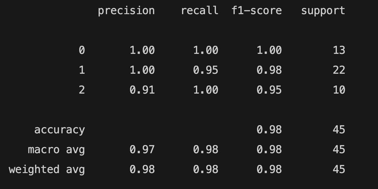
You can check the scikit-learn metrics to learn about metrics.

K-Nearest Neighbors

K-Nearest Neighbors Classifier

K-Nearest Neighbors Classifier is a classification algorithm. Classification is computed from a simple majority vote of the nearest neighbors of each point. You need to specify k, the number of neighbors and the model finds the closest k neighbors. We will use the Wine recognition dataset like in the previous model.

from sklearn.datasets import load_wine
from sklearn.neighbors import KNeighborsClassifier
from sklearn.model_selection import train_test_split

X, y = load_wine(return_X_y=True)

We will split the data and create a KNeighborsClassifier:

X_train, X_test, y_train, y_test = train_test_split(X, y, test_size=0.25, random_state = 27) classifier = KNeighborsClassifier()
classifier.fit(X_train, y_train)
pred = classifier.predict(X_test)

The n_neighbors parameter is used to select the number of neighbors to classify the unknown data. The default value for k is 5. We fit the data and predict X_test. Let's evaluate the model:

from sklearn.metrics import accuracy_score
print(accuracy_score(y_test, pred))

The result is 0.644. We can scale the feature data and change the number of neighbors to improve the model. We can manually change k and calculate the score. However, there's a better way to test different k values:

from sklearn.datasets import load_wine
from sklearn.neighbors import KNeighborsClassifier
from sklearn.preprocessing import StandardScaler
from sklearn.model_selection import train_test_split
from sklearn.metrics import accuracy_score
import matplotlib.pyplot as plt

X, y = load_wine(return_X_y=True)
X_train, X_test, y_train, y_test = train_test_split(X, y, test_size=0.25, random_state = 27)

scaler = StandardScaler()
X_train = scaler.fit_transform(X_train)
X_test = scaler.transform(X_test)

no_of_neighbor = []
scores = []
for k in range(1, 20):
      classifier = KNeighborsClassifier(n_neighbors = k)
      classifier.fit(X_train, y_train)
      pred = classifier.predict(X_test)
      score = accuracy_score(y_test, pred)
      no_of_neighbor.append(k)
      scores.append(score)

plt.plot(no_of_neighbor, scores)
plt.xlabel("number of neighbors")
plt.ylabel("accuracy score")
plt.show()

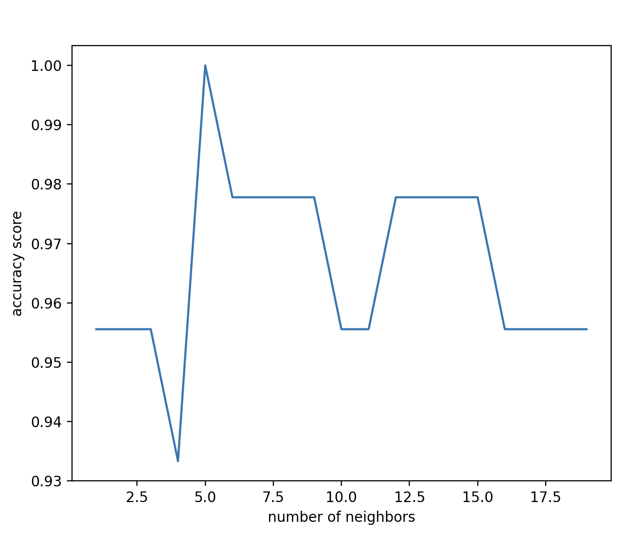
The x-axis in the graph shows the number of neighbors, and y-axis shows the accuracy score. We can use another metric to evaluate our model. We need to select 5 neighbors to get the highest score.

We can use StandardScaler() to scale features. StandardScaler standardizes features by removing the mean and scaling to unit variance. Let's scale the data and change the n_neighbors:

from sklearn.datasets import load_wine
from sklearn.neighbors import KNeighborsClassifier
from sklearn.preprocessing import StandardScaler
from sklearn.model_selection import train_test_split
import matplotlib.pyplot as plt

X, y = load_wine(return_X_y=True)
X_train, X_test, y_train, y_test = train_test_split(X, y, test_size=0.25, random_state = 27)

scaler = StandardScaler()
X_train = scaler.fit_transform(X_train)
X_test = scaler.transform(X_test)

classifier = KNeighborsClassifier(n_neighbors = 5)
classifier.fit(X_train, y_train)
pred = classifier.predict(X_test)

from sklearn.metrics import accuracy_score
print(accuracy_score(y_test, pred))

The new accuracy score is 1.0.

K-Nearest Neighbors Regressor

The K-Nearest Neighbors Regressor is similar to the K-Nearest Neighbors Classifier but used for regression problems. The prediction of the algorithm is the average of the values of k nearest neighbors. We will use fetch_california_housing to fetch scikit-learn's California housing dataset. The default value for the weights parameter is uniform. We chose distance for the weight function to predict. It means closer neighbors of a query point will have a greater influence than neighbors which are further away.

from sklearn.neighbors import KNeighborsRegressor
from sklearn.datasets import fetch_california_housing
from sklearn.model_selection import train_test_split
from sklearn.preprocessing import MinMaxScaler

X, y = fetch_california_housing(return_X_y=True)
X_train, X_test, y_train, y_test = train_test_split(X, y, test_size=0.25, random_state = 20)

scaler = MinMaxScaler()
X_train = scaler.fit_transform(X_train)
X_test = scaler.transform(X_test)

regressor = KNeighborsRegressor(n_neighbors = 7, weights = "distance")
regressor.fit(X_train, y_train)
y_pred = regressor.predict(X_test)

We can evaluate the model using r2_score, mean_squared_error and mean_absolute_error. mean_squared_error is a risk metric corresponding to the expected value of the squared (quadratic) error or loss. mean_absolute_error is a risk metric corresponding to the expected value of the absolute error loss or -norm loss.

from sklearn.metrics import mean_squared_error, mean_absolute_error, r2_score

r2 = r2_score(y_test, y_pred)
print(r2)

mse = mean_squared_error(y_test, y_pred)
print(f"mse: {mse}")

mae = mean_absolute_error(y_test, y_pred)
print(f"mae: {mae}")

0.7085820192410783
mse: 0.40138825542054024
mae: 0.42615182059800666

See scikit-learn metrics for more information.

Decision Tree Classifier

Decision Trees are a non-parametric supervised learning method used for classification and regression. The goal is to create a model that predicts the class (or category) of a target variable by learning simple decision rules inferred from the data features. The scikit-learn's DecisionTreeClassifier module helps to create, train, predict, and visualize a decision tree classifier. We will create a simple pandas DataFrame. The feature columns are "study", "sleep", and "class". "Pass" column has the target values: 1 (Pass) and 0 (Fail).

Decision Tree Classifier Example

from sklearn import tree
import matplotlib.pyplot as plt
from sklearn.tree import DecisionTreeClassifier
from sklearn.model_selection import train_test_split
import pandas as pd

pass_or_not = pd.DataFrame([
      [3, 6, 0, 0],
      [5, 8, 1, 1],
      [4, 5, 0, 0],
      [8, 7, 1, 1],
      [10, 8, 1, 1],
      [6, 4, 0, 0],
      [7, 3, 0, 1],
      [6, 3, 1, 0],
      [5, 8, 0, 0],
      [7, 3, 1, 1],
      [5, 5, 0, 0],
      [4, 7, 1, 0],
      [6, 5, 1, 1],
], columns= ["study", "sleep", "class", "Pass"])

X = pass_or_not.iloc[:, :3 ]
y = pass_or_not["Pass"]

x_train, x_test, y_train, y_test = train_test_split(X,y, random_state=0, test_size=0.2)

"study" shows studying hours, "sleep" shows sleeping hours, and "class" shows if a student attends classes (1 -yes, 0 -no). If the "Pass" value of the student is 1, it means the student passed. If the "Pass" value is 0, the student failed. You can use both numerical and categorical data. However, scikit-learn implementation doesn't support categorical data. Therefore, if you have categorical data, you need to transform the data.

dtree = DecisionTreeClassifier(random_state=12, max_depth=5)
dtree.fit(x_train, y_train)
y_pred = dtree.predict(x_test)

The syntax of DecisionTreeClassifier is similar to previous models. The max_depth parameter shows the maximum depth of the tree. We will plot the tree:

plt.figure(figsize=(10,6))
tree.plot_tree(decision_tree=dtree, feature_names= pass_or_not.columns, class_names={1: "Pass", 0:"Fail"}, filled=True)
plt.tight_layout()
plt.show()

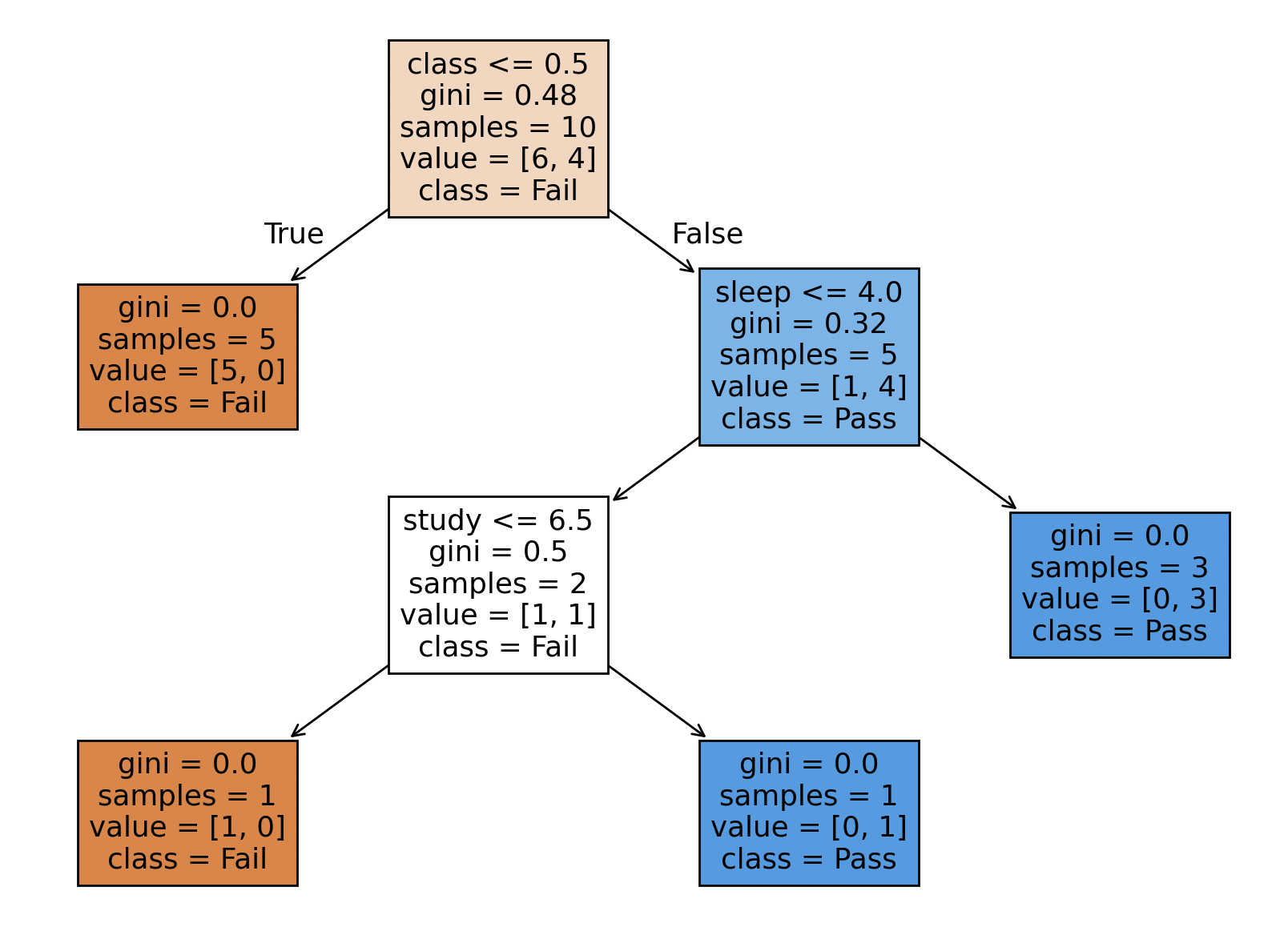
How to interpret the decision tree

A node with no children, which represents the final classification (such as "Pass" or "Fail" in our example), is called a leaf node. The node with no children and the final classification (like "Pass" or "Fail" in our example) is called the leaf node. The first row of the node shows the feature. For example, the splitting feature of the root node is "class <= 0.5". If the feature is true for the sample, you should follow the "True" arrow. Otherwise, you should follow the "False" arrow. The gini shows the impurity at node. If the gini is equal to 0, it's 100% pure (samples belong to the same label/class). The samples value shows the number of samples. The class shows the label/classification.

We can create a DecisionTreeClassifier with scikit-learn's Wine recognition dataset as well:

from sklearn.datasets import load_wine
from sklearn.model_selection import train_test_split
from sklearn.tree import DecisionTreeClassifier
from sklearn import tree
import matplotlib.pyplot as plt

X, y = load_wine(return_X_y=True)
wine = load_wine()
X_train, X_test, y_train, y_test = train_test_split(X, y, test_size=0.25, random_state = 10)

classifier = DecisionTreeClassifier(max_depth=6, max_features=7)
classifier.fit(X_train, y_train)
y_pred = classifier.predict(X_test)
plt.figure(figsize=(10,6))
tree.plot_tree(decision_tree=classifier, feature_names= wine.feature_names, class_names=wine.target_names, filled=True)
plt.tight_layout()
plt.show()

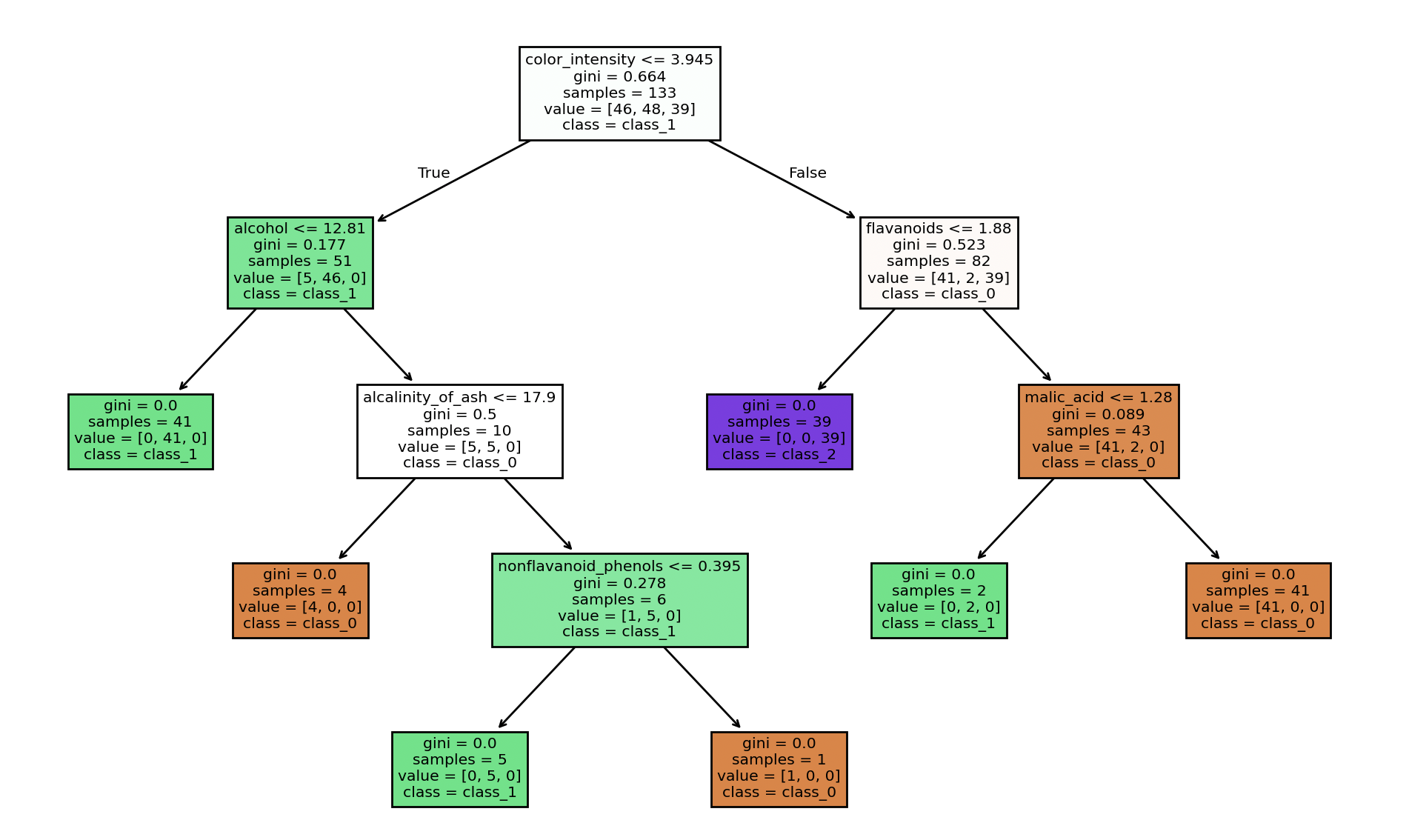
The model is similar to the previous Decision Tree Classifier model. The max_feature parameter limits the number of features. You can check all the DecisionTreeClassifier parameters. You can calculate the accuracy_score of your decision tree.

Interpreting a decision tree can be complicated, you can use the node_ids parameter:

tree.plot_tree(decision_tree=classifier, feature_names= wine.feature_names, class_names=wine.target_names, filled=True, node_ids=True)

The node_ids parameter shows the ID number on each node. If you want to learn more about the decision tree, you can use the tree_ attribute. The tree_ attribute can be used to learn left children, right children, features, threshold, number of training samples reaching node, impurity, weighted number of training samples reaching node and the values:

classifier.tree_.children_left[i]
classifier.tree_.children_right[i]
classifier.tree_.feature[i]
classifier.tree_.threshold[i]
classifier.tree_.n_node_samples[i]
classifier.tree_.impurity[i]
classifier.tree_.weighted_n_node_samples[i]
classifier.tree_.value[i]

If you want to learn the attributes of a specific node, you need to replace i with the node ID. n_node_samples is the number of training samples reaching node i. impurity is the impurity at node i. weighted_n_node_samples is the weighted number of training samples reaching node i. If we train the first model using node_ids parameter, we get the following tree:

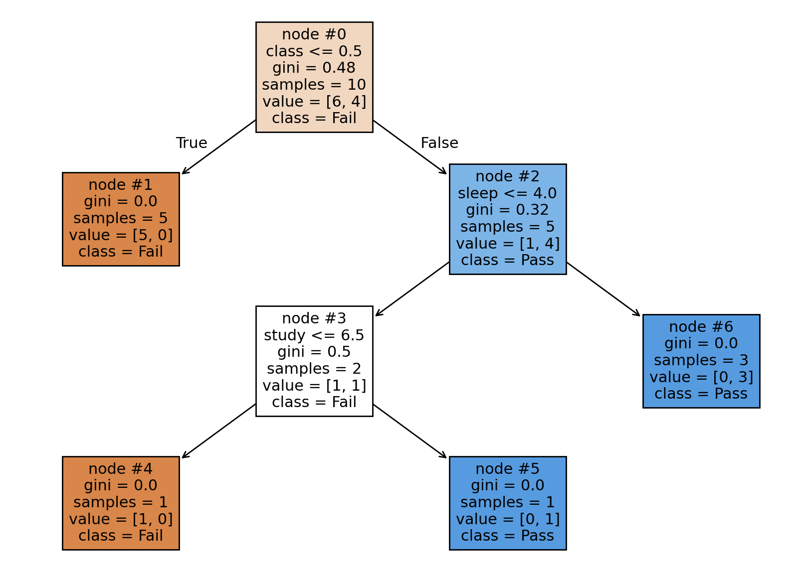
We can check the tree_ attributes of the decision tree above:

print(dtree.tree_.children_left[0])

1

print(dtree.tree_.children_right[1])

-1

print(dtree.tree_.feature[2])

1

print(dtree.tree_.threshold[3])

6.5

print(dtree.tree_.n_node_samples[4])

1

print(dtree.tree_.impurity[5])

0.0

print(dtree.tree_.weighted_n_node_samples[6])

3.0

print(dtree.tree_.value[3])

[[0.5 0.5]]

If you don't specify any node ID ( dtree.tree_.children_left), you can traverse the tree structure and get the left children of the tree.

Preprocessing and Normalization (sklearn.preprocessing)

The sklearn.preprocessing package provides different functions to prepare and transform data for a machine learning model. Normalization is an important process to improve accuracy and performance. For example, features of your data can be on drastically different scales. If you don't normalize them, some features will dominate others. The normalization aims to transform features to be on a similar scale. We used StandardScaler in two different models for two different problems. It was applied to improve convergence in the Logistic Regression model and to enhance accuracy in the K-Nearest Neighbors (KNN) model. Normalization can help models better learn the relative importance (or weights) of each feature. There are different types of scaling methods. We will explore StandardScaler and MinMaxScaler.

StandardScaler

StandardScaler() standardizes features by removing the mean and scaling to unit variance. As mentioned earlier, we used StandardScaler in two different models. It solved the convergence problem in the logistic regression model and improved accuracy in the k-nearest neighbors classification model.

from sklearn.preprocessing import StandardScaler
scaler = StandardScaler()
X = scaler.fit_transform(X)

MinMaxScaler

MinMaxScaler rescales the data set such that all feature values are in the range [0, 1]. We can use MinMaxScaler for the Wine recognition dataset to improve accuracy and get the same result.

from sklearn.preprocessing import MinMaxScaler
scaler = MinMaxScaler()
X = scaler.fit_transform(X)

There are other scalers to normalize data. You can test them and choose the most suitable scaler for your data. See the full list of scikit-learn normalization functions.

Scikit-learn's evaluation metrics

Scikit-learn's Evaluation Metrics For Classification

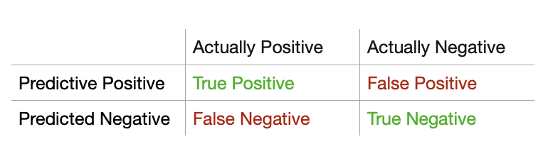
TP = True Positive, TN = True Negative, FP = False Positive, FN = False Negative

You can use the sklearn.metrics module to measure the performance of your module. The sklearn.metrics module offer different metrics to evaluate a classification model. You can check the full list of scikit-learn metrics.

Accuracy Score

The accuracy score is one of the most important metrics for classification models to measure the accuracy of the model, and we already used it in the example.

Accuracy Score = (TP + TN) / (TP + TN + FP + FN)

from sklearn.metrics import accuracy_score
accuracy_score(y_test, y_pred)

The best performance is 1.

Recall Score

Scikit-learn's another evaluation metric for classification is recall.

Recall = TP / (TP + FN)

from sklearn.metrics import recall_score
recall_score(y_test, y_pred)

The best performance is 1, and the worst performance is 0.

Precision score

You can also use precision to measure the performance of your model.

Precision = TP / (TP + FP)

from sklearn.metrics import precision_score
precision_score(y_test, y_pred)

The best performance of precision is 1, and the worst performance is 0.

F1 Score

The F1 score (F-score or F-measure) combines both precision and recall into a single statistic.

F1-Score = (2 x precision x recall) / (precision + recall)

from sklearn.metrics import f1_score
f1_score(y_test, y_pred)

Classification Report

The classification_report is used to build a text report showing the main classification metrics.

from sklearn.metrics import classification_report
classification_report(y_true, y_pred, target_names=target_names)

Using target_names parameter is optional.

You can read the classification report of the logistic regression model that we created.

A classification report displays precision, recall, f1score, accuracy, and support scores of a model. Support refers to the number of actual occurrences of the class in the dataset.

Confusion Matrix

The confusion matrix computes confusion matrix to evaluate the accuracy of a classification.

from sklearn.metrics import confusion_matrix
print(confusion_matrix(y_true, y_pred))

Confusion matrix can be difficult to understand. You can learn how to interpret a confusion matrix with an example.

Scikit-learn's Evaluation Metrics for Regression

sklearn.metrics module has evaluation metrics for regression models as well. We already tested our models using mean_squared_error and mean_absolute_error. mean_squared_error is a non-negative floating point value and the best score is 0.0.
mean_absolute_error is a non-negative floating point value and the best score is 0.0.
Another important evaluation metric is r2_score. r2_score is the regression score function and the best value is 1.0. It can be negative as well.

from sklearn.metrics import mean_squared_error
from sklearn.metrics import mean_absolute_error
from sklearn.metrics import r2_score

mse = mean_squared_error(y_test, y_pred)
mae = mean_absolute_error(y_test, y_pred)
r2 = r2_score(y_test, y_pred)

We imported mean-squared_error, mean_absolute_error, and r2_score separately to show how to import the metrics, but you can import them together: from sklearn.metrics import mean_squared_error, mean_absolute_error, r2_score. If you want to learn other metrics for regression models, read the scikit-learn's metrics page.

Feature selection methods

Feature selection can be helpful to improve efficiency and accuracy. You can remove redundant features and improve your model's performance. There are different feature selection methods. In addition to Scikit-learn's sklearn.feature_selection module, we will use mlxtend library to compare different feature selection methods in the tutorial. Filter methods are provided by the sklearn.feature_selection module. You can use mlxtend's wrapper methods. Scikit-learn also provides embedded methods for feature selection.

Filter Methods

The sklearn.feature_selection module provides different methods for selecting features. You can test the methods below and choose the best feature selection method for your model.

Variance Threshold

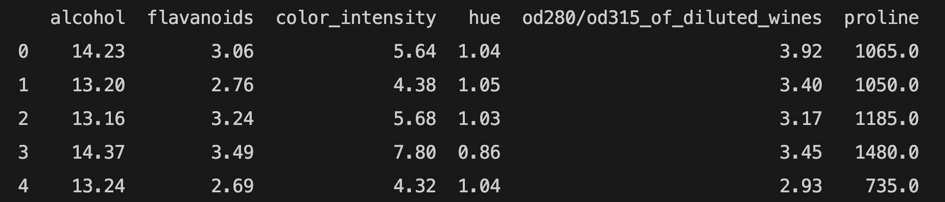
VarianceThreshold is a feature selector that removes all low-variance features. Only features are used in VarianceThreshold; target values are not involved. Therefore, it can be used for unsupervised learning. The method can be used only on numerical values. The threshold parameter represents the threshold that removes the features that have the same or lower value in all samples. The default value is 0. We will be using Scikit-learn's wine dataset.

from sklearn.datasets import load_wine
from sklearn.feature_selection import VarianceThreshold
import pandas as pd

wine = load_wine()
df = pd.DataFrame(wine.data, columns= wine.feature_names)
print(df.columns)

Index(['alcohol', 'malic_acid', 'ash', 'alcalinity_of_ash', 'magnesium', 'total_phenols', 'flavanoids', 'nonflavanoid_phenols', 'proanthocyanins', 'color_intensity', 'hue', 'od280/od315_of_diluted_wines', 'proline'], dtype='object')

X = wine.data
selector = VarianceThreshold(threshold=0.2)
selected = selector.fit_transform(X)
col_names = df.columns[selector.get_support(indices=True)].to_list()
print(col_names)

['alcohol', 'malic_acid', 'alcalinity_of_ash', 'magnesium', 'total_phenols', 'flavanoids', 'proanthocyanins', 'color_intensity', 'od280/od315_of_diluted_wines', 'proline']

We printed the features to see the difference before and after the feature selection. "ash", 'nonflavanoid_phenols', and 'hue' features are removed.

Pearson's Correlation Method

Pandas dataframe.corr() is used to find the pairwise correlation of all columns in the dataset. You can use Pandas corr() method for the correlation among features. For example, if two features are highly correlated, you can remove one of them. You can use the corr() method for the correlation between features and targets. We will use the California housing dataset to see the correlation between features and the target:

from sklearn.datasets import fetch_california_housing
import pandas as pd
import seaborn as sns
import matplotlib.pyplot as plt
housing = fetch_california_housing()

X, y = fetch_california_housing(return_X_y=True)
df = pd.DataFrame(housing.data, columns= housing.feature_names)
df['MedHouseVal'] = y

corr_matrix = df.corr()
corr_target = corr_matrix[['MedHouseVal']].drop(labels=['MedHouseVal'])

sns.heatmap(corr_target, annot=True, cmap='RdBu_r')
plt.title("Housing dataset")
plt.show()

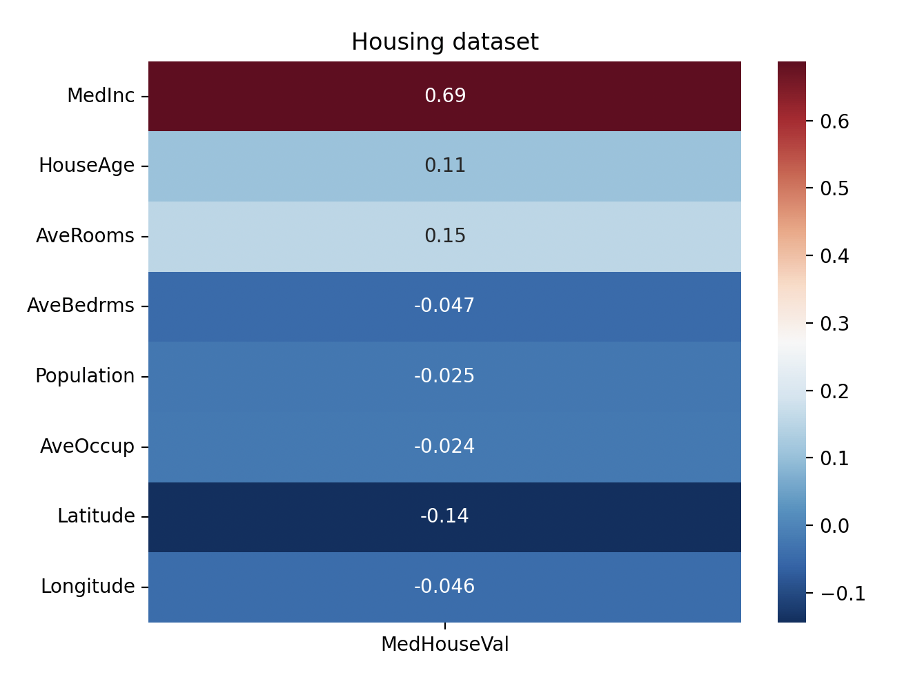
Pearson is the default correlation method. You can use the corr() method only for numerical values. If you have categorical features, you can make the numeric_only parameter True. It will ignore non-numeric values. The dataset we used in the example above has only numerical values.

The heatmap above shows us the correlation between features and target variable. If you want to learn how to make a heatmap, check the seaborn heatmaps. "MedInc" has the highest correlation with the target. "AveOccup" has the lowest correlation with the target. If you want to learn more about the features and the target, you can also calculate f_regression:

from sklearn.feature_selection import f_regression
f_statistic, p_values = f_regression(X, y)

f_regression returns F-statistic and p-values. r_regression is used to calculate f_regression. For more information about r_regression, see r_regression. F-statistics and p-values should be consistent with the Pearson correlation matrix. "MedInc" should have the highest F-statistic and lowest p-value.

SelectKBest

SelectKBest selects features based on the top k highest scores. It takes two main parameters: score_func and k.
score_func is a scoring function that takes two arrays (features and targets) and returns either a single array of scores or a pair of arrays (scores, p-values). The default is f_classif, which is suitable only for classification tasks. You can choose different scoring functions depending on the type of problem. Refer to the available scoring functions in the documentation to choose the right one for your task. k specifies the number of top features to select. The default value is 10. We used the Logistic Regression model with Scikit-learn's wine dataset in the example above. We will use SelectKBest with the same model and the same dataset:

from sklearn.datasets import load_wine
from sklearn.feature_selection import SelectKBest
from sklearn.feature_selection import f_classif, mutual_info_classif
import pandas as pd

X, y = load_wine(return_X_y=True)
wine = load_wine()

df = pd.DataFrame(wine.data, columns= wine.feature_names)
select = SelectKBest(f_classif, k=6)
select.fit_transform(X, y)

We selected (top) 6 features and f_classif for func_score. You can use mutual_info_classif for func_score instead of f_classif. You can see the Logistic Regression example to learn how to calculate the accuracy score.

You can use get_support to print the names of selected features:

features = df[df.columns[select.get_support(indices=True)]]
print(features.head())

Wrapper Methods

Wrapper methods select features by evaluating the performance of models on different subsets of features. In other words, wrapper methods focus on the performance of the model in selecting features. Filter methods do not evaluate the model's performance, they measure the relevance of features. We will use Python's mlxtend library to implement the following wrapper methods: Sequential Forward Selection (SFS), Sequential Backward Selection (SBS), Sequential Forward Floating Selection (SFFS), Sequential Backward Floating Selection (SBFS). You need to install mlxtned library. If you are using pip, run the following command:

pip install mlxtend

If you are using conda, run the following command:

conda install mlxtend

Sequential Feature Selection algorithms aim to select the most relevant features and reduce the number of features. It can improve computational efficiency. Removing irrelevant features can prevent generalization errors as well. Sequential Feature Selection can be used for both classification and regression tasks. We will be using Scikit-learn's wine recognition dataset. The features of the wine recognition dataset are: ['alcohol', 'malic_acid', 'ash', 'alcalinity_of_ash', 'magnesium', 'total_phenols', 'flavanoids', 'nonflavanoid_phenols', 'proanthocyanins', 'color_intensity', 'hue', 'od280/od315_of_diluted_wines', 'proline'].

Sequential Feature Selection Methods

Sequential Forward Selection (SFS) Method

The Sequential Forward Selection (SFS) method starts with no feature and adds one feature at a time. We will be using the Logistic Regression example with wine data. Let's see how Sequential Forward Selection works:

from mlxtend.plotting import plot_sequential_feature_selection as plot_sfs
from mlxtend.feature_selection import SequentialFeatureSelector as SFS
from sklearn.preprocessing import StandardScaler
import matplotlib.pyplot as plt
import pandas as pd
from sklearn.datasets import load_wine
from sklearn.linear_model import LogisticRegression

wine = load_wine()
X = wine.data
y = wine.target

scaler = StandardScaler()
X = scaler.fit_transform(X)
df = pd.DataFrame(X, columns=wine.feature_names)
lr = LogisticRegression(max_iter=300)
sfs = SFS(lr,
        k_features=5,
        forward=True,
        floating=False,
        scoring="accuracy",
        cv=2)
sfs.fit(df, y)
print(sfs.subsets_)

{'feature_idx': (6,), 'cv_scores': array([0.74157303, 0.84269663]), 'avg_score': np.float64(0.7921348314606742), 'feature_names': ('flavanoids',)}
{'feature_idx': (0, 6), 'cv_scores': array([0.88764045, 0.96629213]), 'avg_score': np.float64(0.9269662921348314), 'feature_names': ('alcohol', 'flavanoids')}
{'feature_idx': (0, 6, 12), 'cv_scores': array([0.8988764 , 0.97752809]), 'avg_score': np.float64(0.9382022471910112), 'feature_names': ('alcohol', 'flavanoids', 'proline')}
{'feature_idx': (0, 6, 9, 12), 'cv_scores': array([0.94382022, 0.98876404]), 'avg_score': np.float64(0.9662921348314606), 'feature_names': ('alcohol', 'flavanoids', 'color_intensity', 'proline')}
{'feature_idx': (0, 6, 9, 10, 12), 'cv_scores': array([0.97752809, 0.98876404]), 'avg_score': np.float64(0.9831460674157303), 'feature_names': ('alcohol', 'flavanoids', 'color_intensity', 'hue', 'proline')}

You can follow the selected feature subsets above to understand how Sequential Forward Selection (SFS) works. k_features represents the number of features. As we want to select features by SFS, the forward parameter should be True. The scoring parameter is accuracy. cv parameter is used for cross-validation. If you choose cv=0, you will get the following error: SmallSampleWarning: One or more sample arguments is too small; all returned values will be NaN. See documentation for sample size requirements. Therefore, we chose cv=2.

feature_idx shows the index of feature(s). You can find them in the features list of the wine dataset. feature_names shows the name of the features. cv_score and avg_score represent the cross-validation and average score. We chose 5 features to see the subsets. However, if you want to find the best score, your number of features should be the total number of features for SFS. We can make k=13 and plot a graph for features and their score:

plot_sfs(sfs.get_metric_dict())
plt.show()

We imported plot_sequential_feature_selection from mlxtend.plotting to plot the results. The get_metric_dict() method is used to display the results of feature selection in a pandas DataFrame format for easier visualization and analysis.

The best values for k are 9 and 10 (the avg_score is 0.98) in the example above. After finding the k value for the best score, you can change the k value.

Sequential Forward Floating Selection (SFFS) Method

Sequential Forward Floating Selection (SFFS) is an extension of Sequential Forward Selection (SFS). After each feature is added, SFFS checks whether removing or adding a feature can further improve performance. If performance improves, the change is kept; otherwise, the current feature subset remains unchanged. If you want to use SFFS for feature selection, floating parameter should be True.

Sequential Backward Selection (SBS) Method

Sequential Backward Selection (SBS) method is similar to Sequential Forward Selection. However, Sequential Backward Selection starts with all available features and removes one feature at a time. We will use the previous example to compare Sequential Backward Selection with Sequential Forward Selection.

from mlxtend.plotting import plot_sequential_feature_selection as plot_sfs
import matplotlib.pyplot as plt
import pandas as pd
from sklearn.datasets import load_wine
from sklearn.linear_model import LogisticRegression
from mlxtend.feature_selection import SequentialFeatureSelector as SFS
from sklearn.preprocessing import StandardScaler
from sklearn.datasets import load_wine

wine = load_wine()
scaler = StandardScaler()
X = wine.data
X = scaler.fit_transform(X)
y = wine.target
df = pd.DataFrame(X, columns=wine.feature_names)
lr = LogisticRegression(max_iter=100)
sbs = SFS(lr,
        k_features=5,
        forward=False,
        floating=False,
        scoring='accuracy',
        cv=2)
sbs.fit(df, y)
print(sbs.subsets_)

{13: {'feature_idx': (0, 1, 2, 3, 4, 5, 6, 7, 8, 9, 10, 11, 12), 'cv_scores': array([0.96629213, 0.98876404]), 'avg_score': np.float64(0.9775280898876404), 'feature_names': ('alcohol', 'malic_acid', 'ash', 'alcalinity_of_ash', 'magnesium', 'total_phenols', 'flavanoids', 'nonflavanoid_phenols', 'proanthocyanins', 'color_intensity', 'hue', 'od280/od315_of_diluted_wines', 'proline')},
12: {'feature_idx': (0, 1, 2, 3, 4, 5, 6, 8, 9, 10, 11, 12), 'cv_scores': array([0.97752809, 0.98876404]), 'avg_score': np.float64(0.9831460674157303), 'feature_names': ('alcohol', 'malic_acid', 'ash', 'alcalinity_of_ash', 'magnesium', 'total_phenols', 'flavanoids', 'proanthocyanins', 'color_intensity', 'hue', 'od280/od315_of_diluted_wines', 'proline')},
11: {'feature_idx': (0, 1, 2, 3, 4, 5, 6, 8, 9, 10, 12), 'cv_scores': array([0.97752809, 0.98876404]), 'avg_score': np.float64(0.9831460674157303), 'feature_names': ('alcohol', 'malic_acid', 'ash', 'alcalinity_of_ash', 'magnesium', 'total_phenols', 'flavanoids', 'proanthocyanins', 'color_intensity', 'hue', 'proline')},
10: {'feature_idx': (0, 1, 2, 3, 4, 6, 8, 9, 10, 12), 'cv_scores': array([0.97752809, 1. ]), 'avg_score': np.float64(0.9887640449438202), 'feature_names': ('alcohol', 'malic_acid', 'ash', 'alcalinity_of_ash', 'magnesium', 'flavanoids', 'proanthocyanins', 'color_intensity', 'hue', 'proline')},
9: {'feature_idx': (0, 2, 3, 4, 6, 8, 9, 10, 12), 'cv_scores': array([0.97752809, 0.98876404]), 'avg_score': np.float64(0.9831460674157303), 'feature_names': ('alcohol', 'ash', 'alcalinity_of_ash', 'magnesium', 'flavanoids', 'proanthocyanins', 'color_intensity', 'hue', 'proline')},
8: {'feature_idx': (0, 2, 3, 4, 6, 9, 10, 12), 'cv_scores': array([0.98876404, 0.97752809]), 'avg_score': np.float64(0.9831460674157303), 'feature_names': ('alcohol', 'ash', 'alcalinity_of_ash', 'magnesium', 'flavanoids', 'color_intensity', 'hue', 'proline')},
7: {'feature_idx': (0, 2, 3, 4, 6, 10, 12), 'cv_scores': array([0.98876404, 0.98876404]), 'avg_score': np.float64(0.9887640449438202), 'feature_names': ('alcohol', 'ash', 'alcalinity_of_ash', 'magnesium', 'flavanoids', 'hue', 'proline')},
6: {'feature_idx': (0, 2, 3, 6, 10, 12), 'cv_scores': array([0.98876404, 0.98876404]), 'avg_score': np.float64(0.9887640449438202), 'feature_names': ('alcohol', 'ash', 'alcalinity_of_ash', 'flavanoids', 'hue', 'proline')},
5: {'feature_idx': (0, 2, 6, 10, 12), 'cv_scores': array([0.96629213, 0.96629213]), 'avg_score': np.float64(0.9662921348314607), 'feature_names': ('alcohol', 'ash', 'flavanoids', 'hue', 'proline')}}

The selected feature subsets above show how Sequentail Backward Selection (SBS) works. It removes one feature at a time until it reaches (5 in the example above) the desired number of feature.

We imported plot_sequential_feature_selection from mlxtend.plotting to plot the results. The get_metric_dict() method is used to display the results of feature selection in a pandas DataFrame format for easier visualization and analysis.

plot_sfs(sbs.get_metric_dict())
plt.show()

The best feature selection:

{'feature_idx': (0, 2, 3, 6, 10, 12), 'cv_scores': array([0.98876404, 0.98876404]), 'avg_score': np.float64(0.9887640449438202), 'feature_names': ('alcohol', 'ash', 'alcalinity_of_ash', 'flavanoids', 'hue', 'proline')}

Sequential Backward Floating Selection (SBFS) Method

Sequential Backward Floating Selection (SBFS) is just like Sequential Backward Selection, but after each addition, it checks to see if it can improve performance by removing (or adding) a feature. If the result is better, it removes or adds a feature. Otherwise, the feature subset remains the same. If you want to use SBFS for feature selection, floating parameter should be True.

Recursive Feature Elimination (RFE) Method

Recursive Feature Elimination (RFE) starts by training a model with all available features. RFE ranks all features based on feature importance or model coefficients, then removes the least important feature. This process repeats until the desired number of features—specified by the n_features_to_select parameter—is reached. While RFE is similar to Sequential Backward Selection (SBS), the key difference is that SBS evaluates multiple subsets at each step, whereas RFE trains the model on only a single subset during each iteration. Therefore, RFE is computationally less complex and faster than SBS. You need to import RFE from sklearn.feature_selection module.

from sklearn.feature_selection import RFE
import pandas as pd
from sklearn.datasets import load_wine
from sklearn.linear_model import LogisticRegression
wine = load_wine()
X = wine.data
y = wine.target
names = wine.feature_names
print(wine.feature_names)

['alcohol', 'malic_acid', 'ash', 'alcalinity_of_ash', 'magnesium', 'total_phenols', 'flavanoids', 'nonflavanoid_phenols', 'proanthocyanins', 'color_intensity', 'hue', 'od280/od315_of_diluted_wines', 'proline']

lr = LogisticRegression(max_iter=300)
rfe = RFE(lr, n_features_to_select=6)
rfe.fit(X, y)
print(rfe.ranking_)
print(rfe.support_)
rfe_features = [f for (f, support) in zip(names, rfe.support_) if support]
print(rfe_features)

[1 5 2 3 8 6 1 7 4 1 1 1 1]
[ True False False False False False True False False True True True True]
['alcohol', 'flavanoids', 'color_intensity', 'hue', 'od280/od315_of_diluted_wines', 'proline']

rfe.ranking_ shows the feature rankings. The features with index 1 are kept in the same index. The feature ranking corresponds to the ranking position of the i-th feature. For example, magnesium (ranking feature - 8) is the least important feature and the first feature to be removed.
rfe.support_ shows if the features are selected or removed. If the feature is selected, it returns True. It is consistent with the results of rfe.ranking_ in our example above.
rfe_features shows the selected features after recursive elimination.

If the "ConvergenceWarning: lbfgs failed to converge (status=1): STOP: TOTAL NO. of ITERATIONS REACHED LIMIT." error occurs, you'd better scale your data using StandardScaler instead of increasing max_iter.

Unsupervised Learning in Scikit-learn

Unsupervised Learning is a machine learning model that analyzes unlabeled data. It is used to find patterns and relationships in the data. Clustering and dimensionality reduction are some of the unsupervised machine learning techniques.

K-Means Clustering

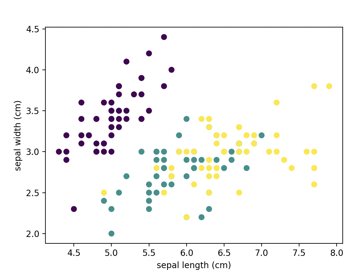
Clustering is a common unsupervised learning technique. K-Means Clustering is an unsupervised machine learning technique that organizes unlabeled data into groups/clusters based on their similarity. K representss the number of clusters in a clustering algorithm; it also refers to the number of centroids to be generated. Means refers to the average distance of data to each cluster center; you should try to minimize it. We'll use Scikit-learn's iris dataset. As there are 3 classes ['setosa', 'versicolor', 'virginica'] in the iris dataset, we will use 3 clusters. We will use the first two features of the iris dataset in the graph. You can use another dataset. If you want to use another dataset and your dataset has many features, you can use one of the feature selection methods we learned.

K-Means Clustering Example

from sklearn.model_selection import train_test_split
from sklearn.datasets import load_iris
from sklearn.cluster import KMeans
import pandas as pd
import matplotlib.pyplot as plt

iris = load_iris()
X,y= load_iris(return_X_y=True)
df = pd.DataFrame(iris.data, columns= iris.feature_names)
target = iris.target

model = KMeans(n_clusters=3, random_state=0)
model.fit(X)
labels = model.predict(X)
plt.scatter(X[:,0], X[:,1], c=target)
plt.xlabel("sepal length (cm)")
plt.ylabel("sepal width (cm)")
plt.show()

Elbow method

If you're unsure about the number of clusters, you can use the elbow method. The elbow method is a graphical method for finding the optimal K value in a k-means clustering algorithm. This method relies on the Within-Cluster Sum of Squares (WCSS), which measures the total squared distance between each point in a cluster and its corresponding centroid. Let's try the elbow method for Scikit-learn's iris dataset:

num_clusters = [1,2,3,4,5,6,7,8]
inertias = []
features = iris.data

for i in num_clusters:
      model = KMeans(n_clusters=i)
      model.fit(features)
      inertias.append(model.inertia_)

plt.plot(num_clusters, inertias, '-o')
plt.xlabel('Number of Clusters (k)')
plt.ylabel('Inertia')
plt.show()

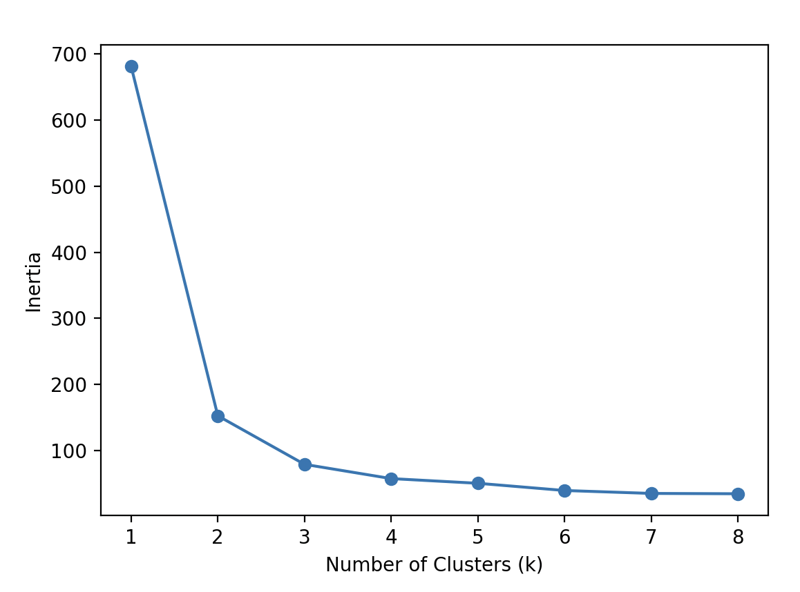
Inertia is the distance from each sample to the centroid of its cluster. The optimal K value for our example is 3 because the rate of decrease in inertia starts to slow down at 3.

Limitations of K-Means Clustering

K-Means clustering has some limitations and may not always be the best choice for your data. For example, the accuracy score in the previous example above was very low, and your model might face similar issues. Therefore, it's important to keep these limitations in mind:

• K-Means is sensitive to the initial placement of cluster centers.
• Choosing the optimal value of K is crucial.
• It assumes clusters are spherical (round) and roughly the same size.
• Outliers can negatively impact the results.

If your data meets the assumptions, K-Means is likely to perform well.

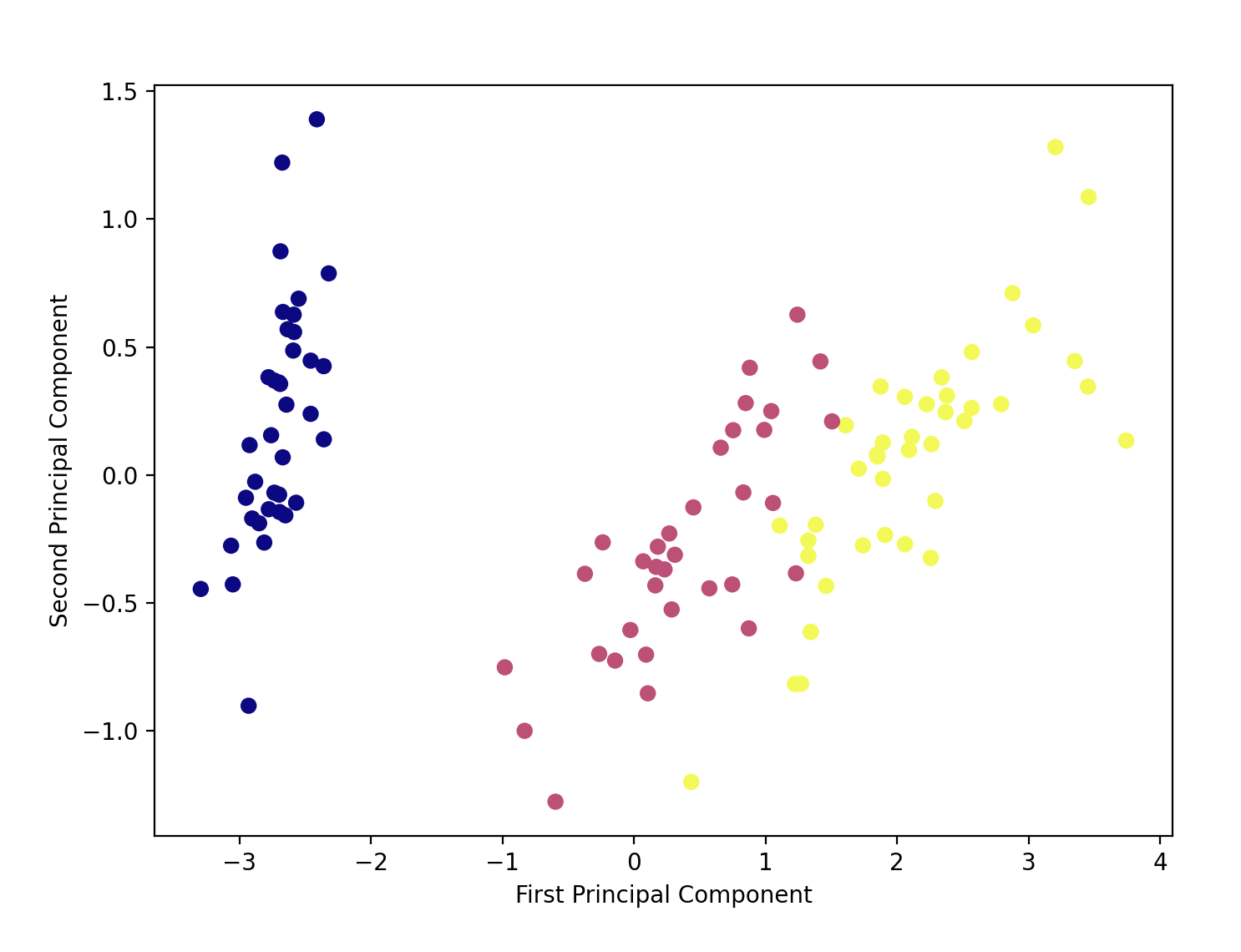
Principal Component Analysis (PCA)

Principal Component Analysis (PCA) is a linear dimensionality reduction technique that uses Singular Value Decomposition (SVD) to project data into a lower-dimensional space. It's a common unsupervised learning technique for large datasets. Despite dimensionality reduction, it retains the essential data. The input data is centered but not scaled for each feature before applying LogisticRegression. We will use Scikit-learn's iris dataset to compare the results with K-Means Clustering.

Principal Component Analysis (PCA) Example

from sklearn.metrics import accuracy_score
from sklearn.linear_model import LogisticRegression
from sklearn.model_selection import train_test_split
from sklearn.datasets import load_iris
from sklearn.decomposition import PCA
import matplotlib.pyplot as plt

X, y = load_iris(return_X_y=True)
X_train, X_test, y_train, y_test = train_test_split(X, y, test_size=0.25, random_state = 20)

pca = PCA(n_components=2)
X_train = pca.fit_transform(X_train)
X_test = pca.transform(X_test)

lr = LogisticRegression()
lr.fit(X_train, y_train)
y_pred = lr.predict(X_test)
print(accuracy_score(y_test, y_pred))

The accuracy score is 0.94. You can learn singular values:

print(pca.singular_values_)

[21.94910388 5.31925179]

We can also visualize the PCA algorithm:

plt.figure(figsize=(8, 6))
plt.scatter(X_train[:,0], X_train[:,1], c=y_train, cmap='plasma')
plt.xlabel('First Principal Component')
plt.ylabel('Second Principal Component')
plt.show()

Supervised Learning II

Naive Bayes Classifier

The Naive Bayes is a supervised learning method based on applying the theorem of Bayes with strong feature independence assumptions to make predictions and classifications. There are different Naive Bayes methods. We will explore Scikit-learn's MultinomialNB classifier and GaussianNB algorithm. If you want to learn Scikit-learn's other Naive Bayes classifiers, see the sklearn.naive_bayes page. We will have a quick review of the Bayes Theorem:

P(A) and P(B) are the probabilities of events A and B
P(A|B) is the probability of event A when event B occurs
P(B|A) is the probability of event B when event A occurs
P(A∩B)=P(A) * P(B)
P(A|B)= P(B|A) * P(A) | P(B)

The Naive Bayes Theorem assumes that features are independent.

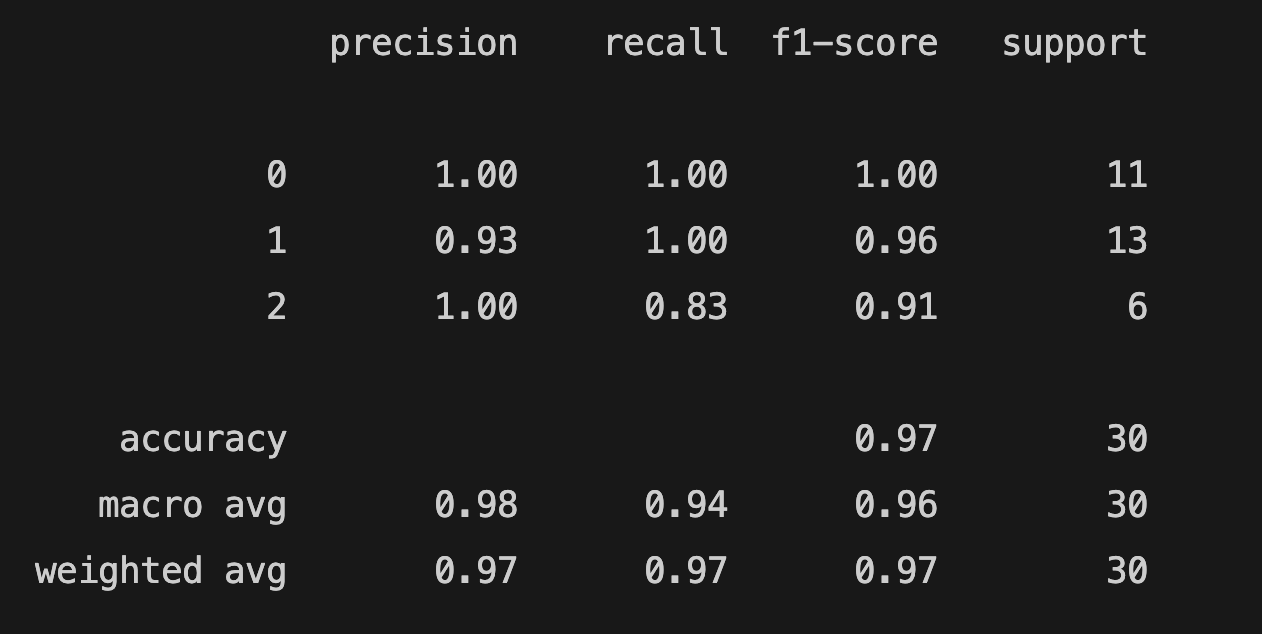
Gaussian Naive Bayes is suitable for continuous data, especially when the features follow a Gaussian (normal) distribution. We will apply GaussianNB on iris data:

Naive Bayes Classifier Example

from sklearn.model_selection import train_test_split
from sklearn.naive_bayes import GaussianNB
from sklearn.datasets import load_iris
from sklearn.metrics import classification_report

X, y = load_iris(return_X_y=True)
X_train, X_test, y_train, y_test = train_test_split(X, y, test_size=0.2, random_state=0)

gnb = GaussianNB()
gnb.fit(X_train, y_train)
y_pred = gnb.predict(X_test)

from sklearn.metrics import accuracy_score
print(accuracy_score(y_test, y_pred))
print(classification_report(y_test, y_pred))

The accuracy score is 0.96.

You can find the model's predicted target values (PTV) and the estimated target values (ETV) below. We can use sklearn's confusion_matrix and ConfusionMatrixDisplay to calculate and display the confusion matrix:

print(f"PTV: {y_test}")
print(f"ETV: {y_pred}")

PTV: [2 1 0 2 0 2 0 1 1 1 2 1 1 1 1 0 1 1 0 0 2 1 0 0 2 0 0 1 1 0]
ETV: [2 1 0 2 0 2 0 1 1 1 1 1 1 1 1 0 1 1 0 0 2 1 0 0 2 0 0 1 1 0]

[[ 11 0 0]
[ 0 13 0]
[ 0 1 5]]

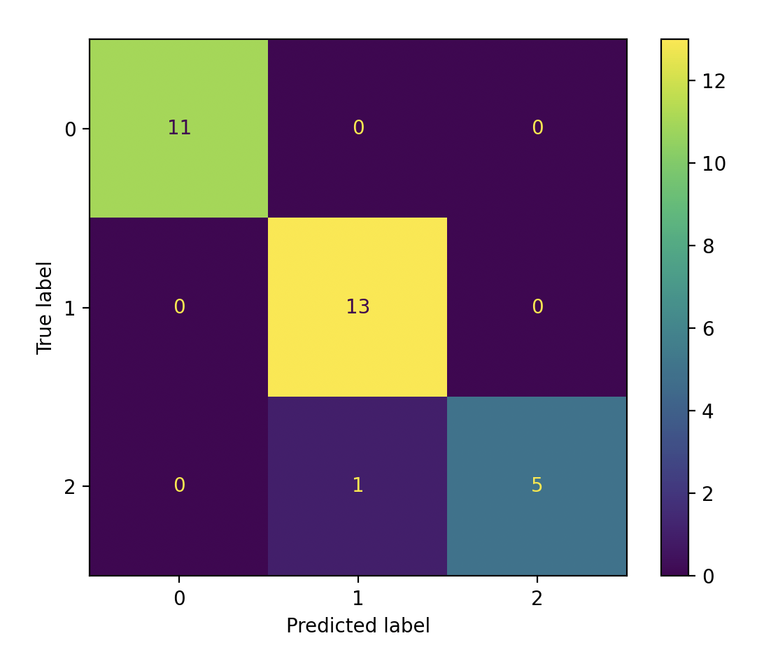
If you want to learn how to interpret the confusion matrix, see the Scikit-learn's confusion matrix.

MultinomialNB

MultinomialNB is a Naive Bayes classifier for multinomial models. The multinomial Naive Bayes classifier is suitable for classification with discrete features. We will use Scikit-learn's MultinomialNB for text classification. We also need to use CountVectorizer to convert text data into numerical features for text classification tasks.

from sklearn.feature_extraction.text import CountVectorizer
from sklearn.naive_bayes import MultinomialNB
from sklearn.model_selection import train_test_split
import pandas as pd
import numpy as np

We will use positive and negative hotel reviews for text classification. Our data below have text and review features. Positive reviews are represented by 1; negative reviews are represented by 0.

reviews = [{"text": "Loved everything about this hotel!", "review": 1},
{"text": "Beds were super comfy", "review": 1},
{"text": "Room came with complimentary snacks", "review": 1},
{"text": "Perfect", "review": 1},
{"text": "Very good", "review": 1},
{"text": "Superb", "review": 1},
{"text": "Breakfast was excellent", "review": 1},
{"text": "Highly recommended", "review": 1},
{"text": "Great breakfast", "review": 1},
{"text": "My room was dirty", "review": 0},
{"text": "Too expensive", "review": 0},
{"text": "Rooms are old", "review": 0},
{"text": "The air condition wasn't working", "review": 0},
{"text": "The hotel was too noisy", "review": 0},
{"text": "Location was great", "review": 1},
{"text": "Rude staff", "review": 0},
{"text": "Unpleasant Room smell", "review": 0},
{"text": "Uncomfortable bed", "review": 0},
{"text": "Overpriced room", "review": 0},
{"text": "Exceptional", "review": 1},
]

We will create two separate lists: one for positive adjectives and another for negative adjectives used in hotel reviews. The model will use positive and negative lists to decide whether reviews are negative or positive.

negative = ["terrible", "horrible", "painful", "disgusting", "boring", "disappointing", "bad", "dirty", "old", "rude", "uncomfortable", "overpriced"]
positive = ["classic", "great", "awesome", "hilarious", "sensitive", "powerful", "heartwarming", "breathtaking", "epic", "thrilling", "best", "good", "exceptional"]

list = pd.DataFrame(reviews)
comments = list.get("text")
comments = np.array(comments)
labels = list.get("review")
labels = np.array(labels)

counter = CountVectorizer()
counter.fit(negative + positive)
review_counts = counter.transform(comments)
training_counts = counter.transform(negative + positive)
training_labels = [0] * 12 + [1] * 13

classifier = MultinomialNB()
classifier.fit(training_counts, training_labels)
rev_counts = counter.transform(comments)

y_pred = classifier.predict(rev_counts)
y_proba = classifier.predict_proba(rev_counts)

from sklearn.metrics import accuracy_score
print(accuracy_score(labels, y_pred))
print(y_proba)

The accuracy score is 0.8.

[[0.48 0.52 ]
[0.48 0.52 ]
[0.48 0.52 ]
[0.48 0.52 ]
[0.32157969 0.67842031]
[0.48 0.52 ]
[0.48 0.52 ]
[0.48 0.52 ]
[0.32157969 0.67842031]
[0.65470208 0.34529792]
[0.48 0.52 ]
[0.65470208 0.34529792]
[0.48 0.52 ]
[0.48 0.52 ]
[0.32157969 0.67842031]
[0.65470208 0.34529792]
[0.48 0.52 ]
[0.65470208 0.34529792]
[0.65470208 0.34529792]
[0.32157969 0.67842031]]

The predict_proba method returns probability estimates for the test vector X. For example, if the probabilities for the first review are [0.48, 0.52], the first number (0.48) represents the probability that the review is class 0 (negative), and the second number (0.52) represents the probability that it is class 1 (positive). Since 0.52 is higher, the model predicts the review as positive.
In summary, predict_proba returns class probabilities, while predict returns the final predicted class based on those probabilities.

We can evaluate our model with another important classification metric: the confusion matrix. The confusion matrix computes the confusion matrix to evaluate the accuracy of a classification.

from sklearn.metrics import confusion_matrix
print(confusion_matrix(labels, y_pred))

[[ 5 4]
[ 0 11]]

The interpretation of the Scikit-learn's confusion matrix can be confusing. The Scikit-learn's confusion matrix in binary classification is formulated as follows: the count of true negatives is C_0,0, false negatives is C_1,0, true positives _1,1, and false positives C_0,1. If you need to review the terms, you can check the table. Let's remember the estimated target values (ETV) and correct target values (CTV) to understand the confusion matrix above:

ETV: [1 1 1 1 1 1 1 1 1 0 1 0 1 1 1 0 1 0 0 1]
CTV: [1 1 1 1 1 1 1 1 1 0 0 0 0 0 1 0 0 0 0 1]

You should keep in mind that scikit-learn's confusion_matrix is different from the classification_report in the evaluation metrics. In our example, we labeled negative reviews as 0 and positive reviews as 1, meaning that 0 represents negative sentiment and 1 represents positive sentiment. The total number of true negatives—cases where both the actual and predicted labels are 0—is 5 in this case. This value appears in the confusion matrix at position [0, 0], which corresponds to row 0 and column 0.
If your model is performing multiclass classification, the structure of the confusion matrix follows a consistent pattern: the rows represent the true (actual) target values in ascending order, and the columns represent the predicted target values, also in ascending order from left to right.
You can visualize the confusion matrix using ConfusionMatrixDisplay, as shown in the example above.

from sklearn.metrics import confusion_matrix, ConfusionMatrixDisplay
import matplotlib.pyplot as plt

cm = confusion_matrix(labels, y_pred, labels=classifier.classes_)
disp = ConfusionMatrixDisplay(confusion_matrix=cm, display_labels=classifier.classes_)
disp.plot()
plt.show()

You can also see the confusion matrix of the previous (GaussianNB) example using iris data for multiclass classification.

If the number of True Positives and False Negatives (TP + FN) is equal to 0, you will get the following warning: "UndefinedMetricWarning: Precision is ill-defined and being set to 0.0 in labels with no predicted samples. Use `zero_division` parameter to control this behavior." You need to use the zero_division parameter to set a value to return when there is a zero division.

classification_report(labels, y_pred, zero_division=0)

Support Vector Machines (SVM)

The Support Vector Machine (SVM) is another important supervised machine learning model used for classification and regression tasks. A SVM defines a decision boundary using labeled data to classify unlabeled points. The distance between the support vectors and the decision boundary is called the margin. The support vectors are the points in the training set closest to the decision boundary. If there are n number of features, there should be n+1 support vectors. Scikit-learn's sklearn.svm offers support vector machine algorithms, and we will use SVC, Support Vector Classifier (C-Support Vector Classification). SVC is a powerful algorithm and it's easy to use. The implementation is based on libsvm. Let's see how to make a model with SVC:

Support Vector Machines (SVM) Example

import numpy as np
from sklearn.datasets import load_wine
from sklearn.preprocessing import StandardScaler
from sklearn.model_selection import train_test_split
from sklearn.svm import SVC

X,y = load_wine(return_X_y=True)
X_train, X_test, y_train, y_test = train_test_split(X, y, test_size=0.2, random_state=0)
scaler = StandardScaler()
X_train = scaler.fit_transform(X_train)
X_test = scaler.transform(X_test)

classifier = SVC(kernel="rbf", gamma =0.1)
classifier.fit(X_train, y_train)
y_pred = classifier.predict(X_test)

from sklearn.metrics import accuracy_score
print(accuracy_score(y_test, y_pred))

The accuracy_score is 1.

We split and scale the data in the Support Vector Machine example above. We create an SVC object. We used kernel and gamma parameters. The kernel parameter specifies the kernel type to be used in the algorithm. The default value is "rbf". We mentioned earlier that the number of features (and the distribution of data) is important in SVM. SVM aims to find the optimal hyperplane to separate data and maximize the margin to prevent false classification. Therefore, the kernel parameter offers the following kernel types: "linear", "poly", "rbf", "sigmoid", and "precomputed". The kernel transforms the data into a higher dimension. The polynomial kernel uses the polynomial function, while the rbf kernel uses the Radial Basis Function to transform data into a higher dimension. The rbf kernels are used when the data is unevenly distributed. Before explaining gamma, we'll explore the C parameter. The C parameter is the regularization parameter of SVM and is used to control misclassification. In other words, it is the cost of misclassification. The strength of the regularization is inversely proportional to C. The default value is 1.0, and we didn't change it. If C is small, the SVM has a soft margin. Although the margin is large, there will be classification errors. The gamma parameter is similar to the C parameter. The gamma parameter is the kernel coefficient for "rbf", "poly", and "sigmoid". It can be "scale", "auto", or "float" (but not negative). If the gamma is large, the model is more sensitive to the changes in training data.

You can learn the support vectors using the support_vectors attribute:

print(classifier.support_vectors_)

Linear Discriminant Analysis (LDA)

Linear discriminant analysis (LDA) is a dimensionality reduction technique used in classification problems. It is similar to Principal Component Analysis (PCA), but LDA is a supervised learning machine technique. LDA maximizes the distance between classes and minimizes the distance within each class. We will use Scikit-learn's sklearn.discriminant_analysis module. According to Scikit-learn, sklearn.discriminant_analysis is a classifier with a linear decision boundary, generated by fitting class conditional densities to the data and using Bayes' rule. It assumes that all classes share the same covariance matrix, and the model fits a Gaussian density to each class. Let's see how to use sklearn.discriminant_analysis:

Linear Discriminant Analysis (LDA) Example

from sklearn.discriminant_analysis import LinearDiscriminantAnalysis
from sklearn.datasets import load_wine
from sklearn.linear_model import LogisticRegression
from sklearn.model_selection import train_test_split
from sklearn.preprocessing import StandardScaler

X, y = load_wine(return_X_y=True)
X_train, X_test, y_train, y_test = train_test_split(X, y, test_size=0.30, random_state = 20)

scaler = StandardScaler()
X_train = scaler.fit_transform(X_train)
X_test = scaler.transform(X_test)

lda = LinearDiscriminantAnalysis(n_components= 2)
X_train = lda.fit_transform(X_train, y_train)
X_test = lda.transform(X_test)

lr = LogisticRegression()
lr.fit(X_train, y_train)
y_pred = lr.predict(X_test)

from sklearn.metrics import accuracy_score
print(accuracy_score(y_test, y_pred))

The score is 0.98. The n_components is 2 because there are 3 classes in the wine dataset, and it should be n_classes - 1. As mentioned earlier, LDA has some assumptions. The number of the smallest class should be greater than the number of variables as well. LDA is a powerful dimensionality reduction technique, but your data should meet the assumptions.

Next Steps

You've now covered the fundamentals and important methods. To explore advanced concepts in more depth, refer to our separate articles on advanced Scikit-learn topics.